Master VLOOKUP Multiple Criteria and Advanced Formulas Smartsheet
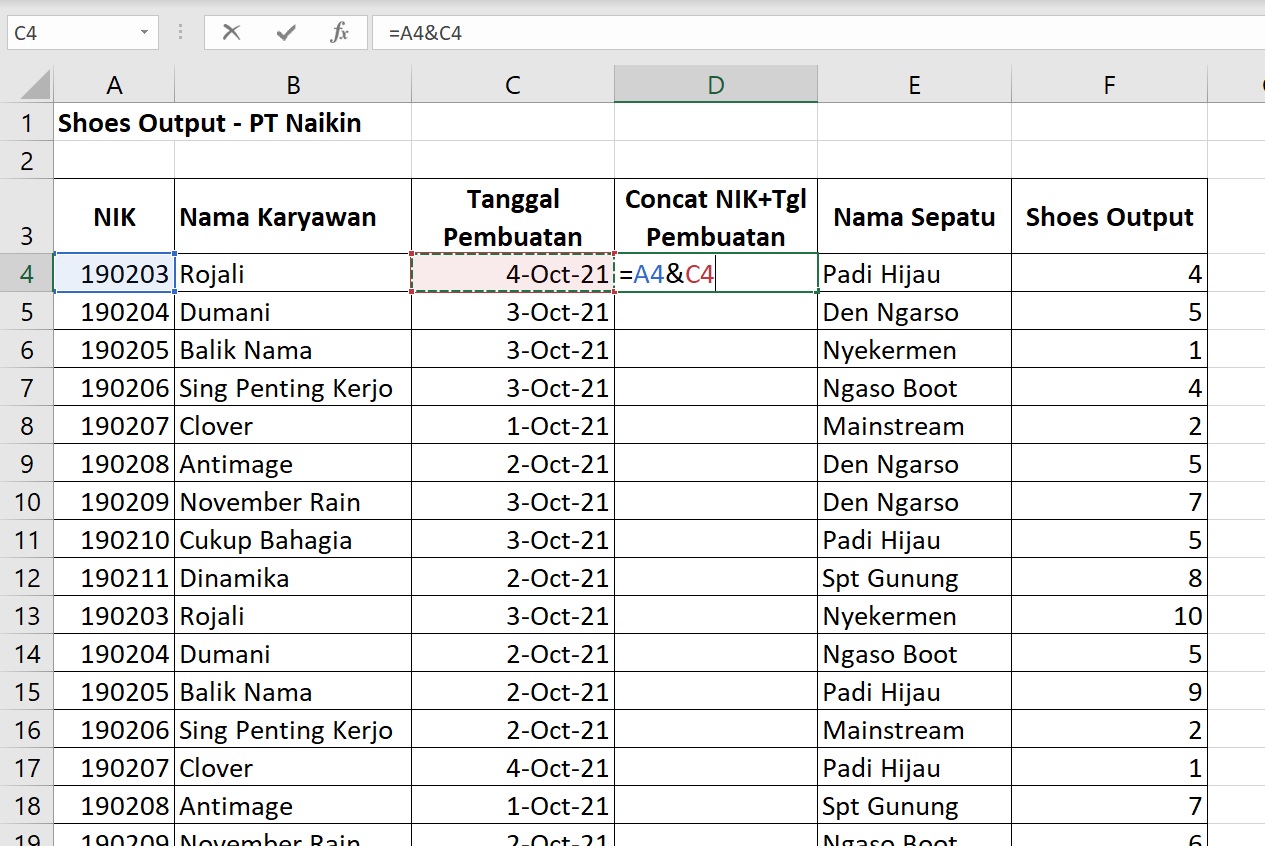
Enter =VLOOKUP in cell B4, which is the first cell in the column. Enter C4, the first value (Adams) you want to use as criteria. Enter & to combine two values. Enter D4, the second value (Presley) you want to use as criteria. Drag the formula down to combine the values for each row. Enter =VLOOKUP in cell H5, where you want the Email address to.

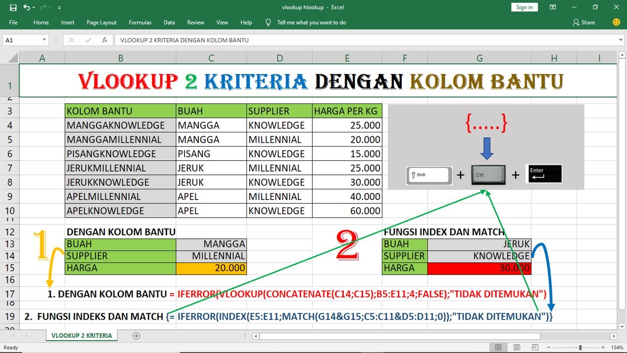
VLOOKUP 2 DAN 3 KRITERIA Tutorial Pemula Excel YouTube
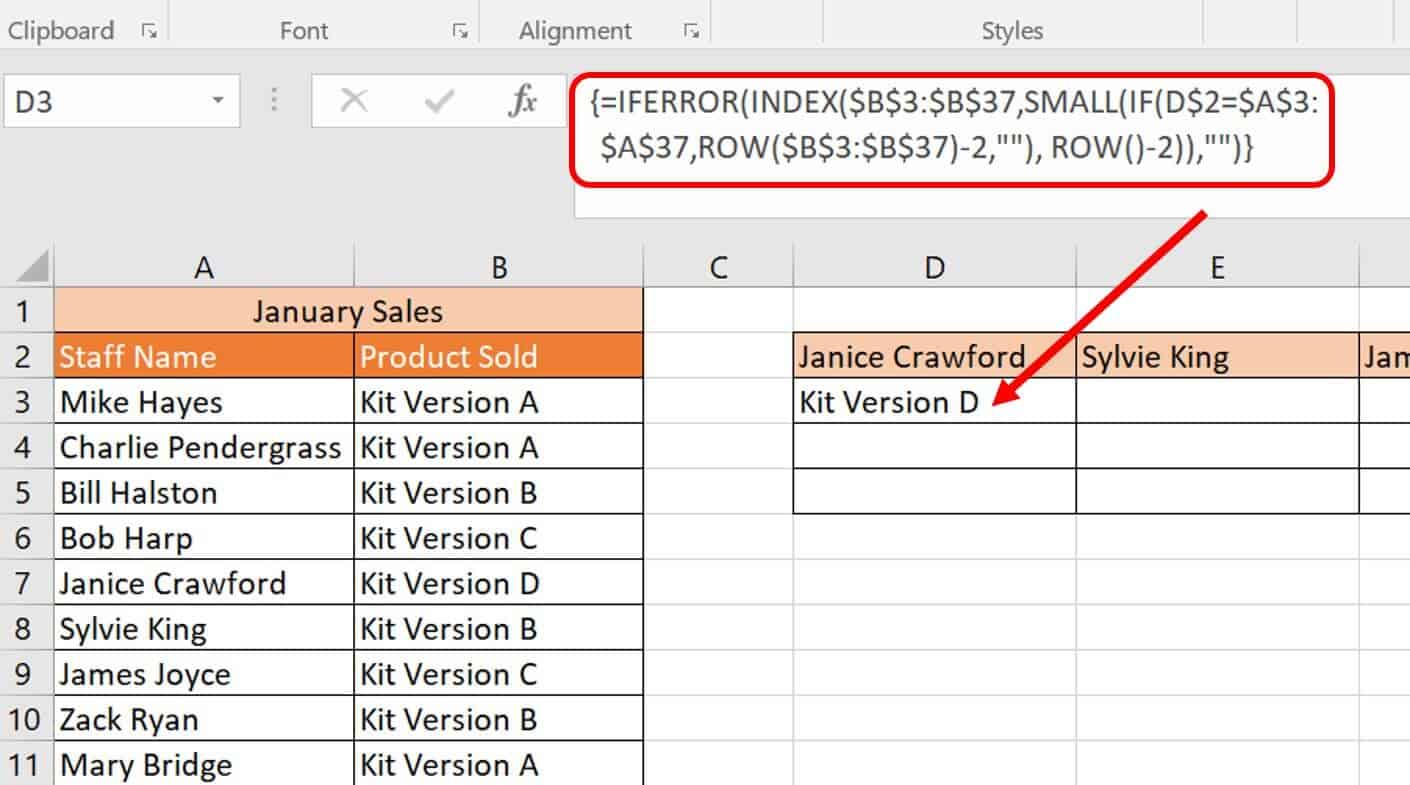
Joining VLOOKUP with MATCH Function to Include Multiple Criteria in Excel The MATCH function returns a relative position of an item in an array that matches a specified value in a specified order. By combining the VLOOKUP with the MATCH function here, we can specify the output types manually. The required formula in Cell C18 will be now:
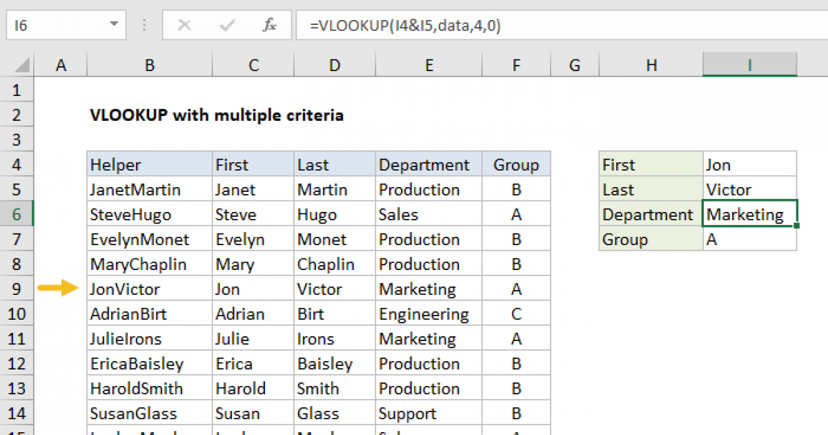
VLOOKUP with multiple criteria Excel formula Exceljet
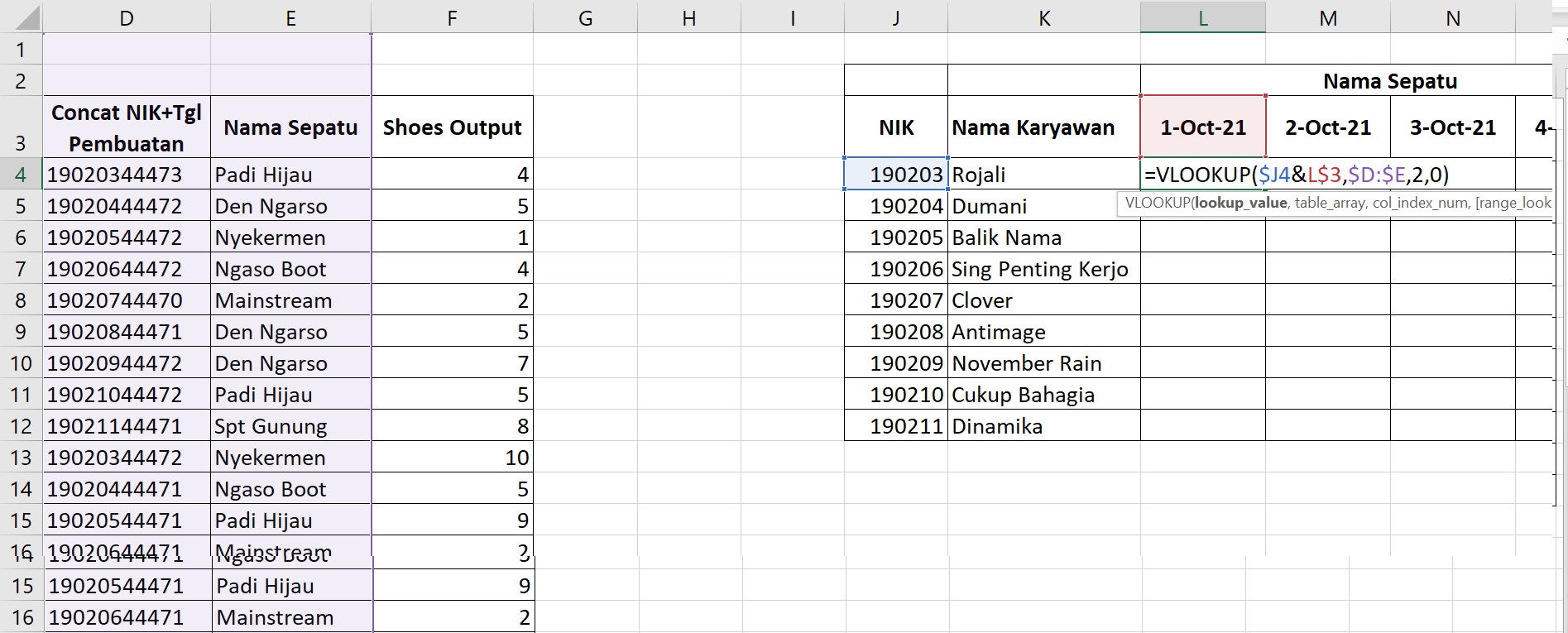
Here are the steps: Insert a Helper Column between column B and C. Use the following formula in the helper column: =A2&"|"&B2 This would create unique qualifiers for each instance as shown below. Use the following formula in G3 =VLOOKUP ($F3&"|"&G$2,$C$2:$D$19,2,0) Copy for all the cells. How does this work?
Rumus Vlookup Dengan 2 Kriteria Di Excel Vrogue
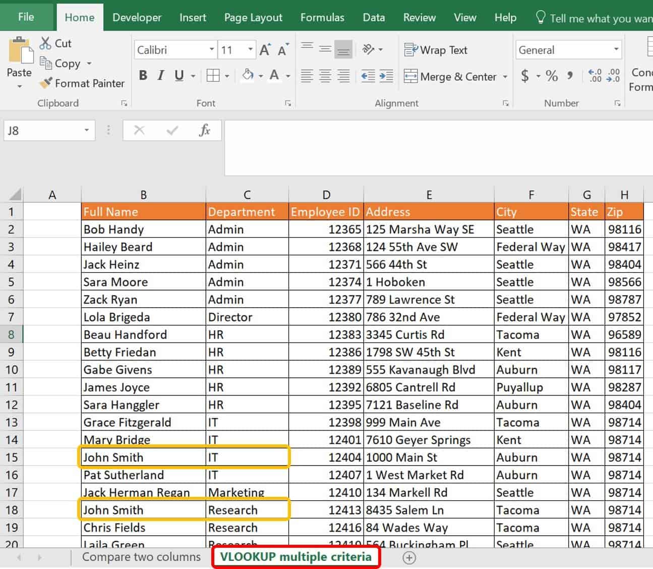
Recommended Articles VLOOKUP Formula in Excel Let us now see examples of the VLOOKUP function with multiple criteria search. You can download this VLOOKUP with Multiple Criteria template here - VLOOKUP with Multiple Criteria template Example #1 Suppose you have data of employees of your company.

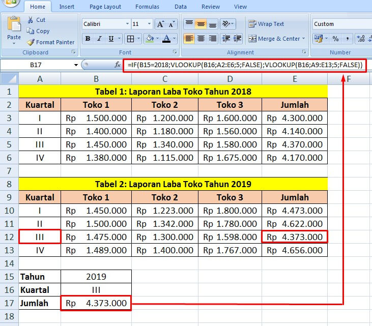
Tutorial EXCEL Kombinasi Rumus VLOOKUP dan IF VLOOKUP 2 Kriteria atau Lebih YouTube
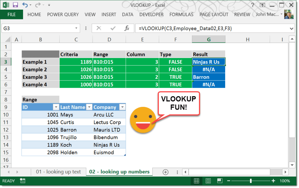
A logical value that specifies whether you want VLOOKUP to find an approximate or an exact match: Approximate match - 1/TRUE assumes the first column in the table is sorted either numerically or alphabetically, and will then search for the closest value. This is the default method if you don't specify one. For example, =VLOOKUP(90,A1:B100,2,TRUE).
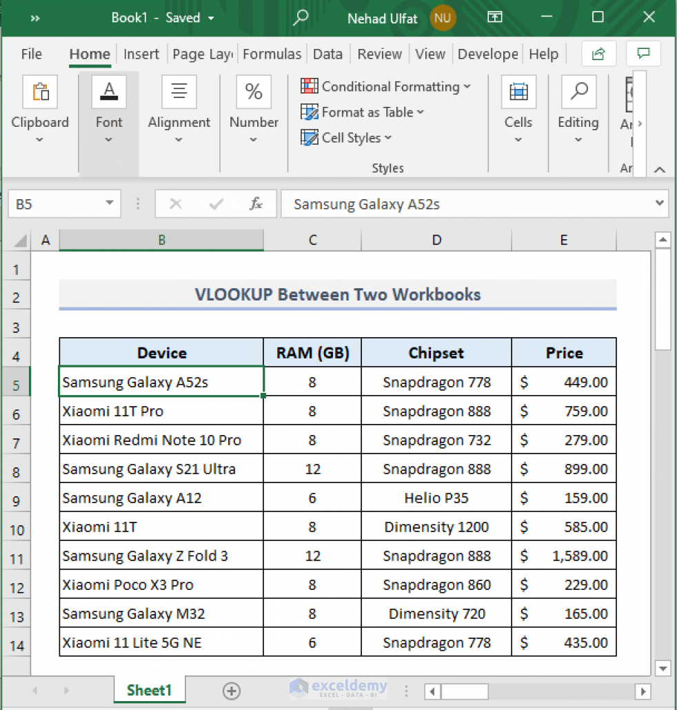
VLOOKUP Example Between Two Sheets in Excel
While using the VLOOKUP function in Excel, we will often need to lookup a value based on two criteria. This is possible by modifying the lookup value in the standard VLOOKUP function. In this tutorial, we will learn how to apply VLOOKUP with two criteria. Figure 1. Final result Syntax of the VLOOKUP formula
VLOOKUP dengan 2 KRITERIA pada kolom yang berbeda YouTube
Method-3: Combining VLOOKUP and MATCH Functions. Another way to use VLOOKUP with multiple criteria in different columns involves using the MATCH function. Now, the MATCH function returns the relative position of an item matching a specific value in an array, therefore, let's see it in action. 📌 Steps:

Vlookup 2 Kriteria Row dan Column Excel YouTube
Excel VLOOKUP Two Criteria allows the user to look up values based on two criteria, thus making it easier to find specific information in large data sets. To perform this function, the user must first define the lookup value and specify the table array range where the data is located.
Excel4Work VLOOKUP dengan 2 Kriteria , Emang bisa?
1. Click on the SUMPRODUCT-multiple_criteria worksheet tab in the VLOOKUP Advanced Sample file. This worksheet tab has a portion of staff, contact information, department, and ID numbers. In this example, let's use the criteria of Full Name and Department to look for an employee's ID number. 2.

Vlookup Dengan 2 Kriteria
2. Excel VLOOKUP with CHOOSE Function to Add Multiple Criteria in Column and Row. If you want to avoid the Helper column, then, this example will certainly help you.We can use the CHOOSE function with the VLOOKUP function to add multiple criteria in columns and rows. The CHOOSE function chooses a value or action to perform from a list of values based on an index number.
Master VLOOKUP Multiple Criteria and Advanced Formulas Smartsheet
VLOOKUP on Two or More Criteria Columns Jeff Lenning | January 10, 2014 | 47 Comments | CONCATENATE, SUMIFS, VLOOKUP If you have ever tried to use a VLOOKUP function with two or more criteria columns, you've quickly discovered that it just wasn't built for that purpose.
Excel4Work VLOOKUP dengan 2 Kriteria , Emang bisa?
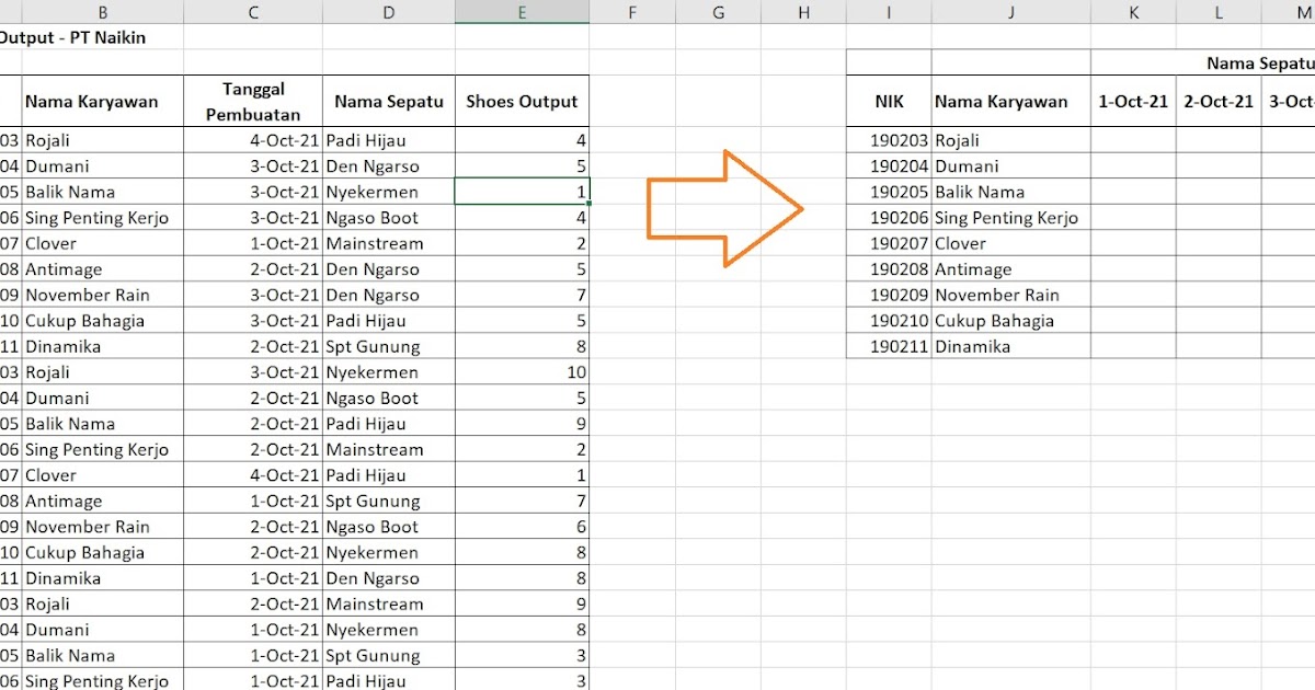
Vlookup 2 kriteria - Pada dasarnya fungsi atau rumus Vlookup excel hanya bisa melakukan pencarian data dengan 1 kriteria atau 1 kata kunci. Itupun dengan syarat bahwa data yang dicari berada di kolom pertama tabel referensi pencarian.
Excel4Work VLOOKUP dengan 2 Kriteria , Emang bisa?
by Svetlana Cheusheva, updated on March 22, 2023 These examples will teach you how to Vlookup multiple criteria, return a specific instance or all matches, do dynamic Vlookup in multiple sheets, and more. It is the second part of the series that will help you harness the power of Excel VLOOKUP.

Vlookup dan hlookup dua kriteria Tutorial Microsoft Excel YouTube
Step 1: Set Up the Multiple Conditions. Step 1 Example. Step 2: Use the FILTER Function to Extract the Value (s) in the Row Where the Multiple Conditions are Met. Step 2 Example. Download the VLookup Multiple Criteria (with the FILTER Function) Example Workbook. Related Excel Training Materials and Resources.
VLOOKUP function How To Excel
To apply multiple criteria with the VLOOKUP function you can use Boolean logic and the CHOOSE function. In the example shown, the formula in H8 is: =VLOOKUP(1,CHOOSE({1,2},(H5=data[Item])*(H6=data[Size])*(H7=data[Color]),data[Price]),2,0) where "data" is an Excel Table in B5:E15. The result is $30.00, the price of a Large Red Hoodie. This is an array formula, and must be entered with control.
VLOOKUP 2 Kriteria di Microsoft eXcel YouTube
Step 4: Enter the Formula as an Array Formula. The VLookup multiple criteria (with INDEX MATCH) formula template/structure you learned in this Tutorial is an array formula. If you're working with Excel 2019 or earlier, enter this VLookup multiple criteria (with INDEX MATCH) formula by pressing "Ctrl + Shift + Enter".