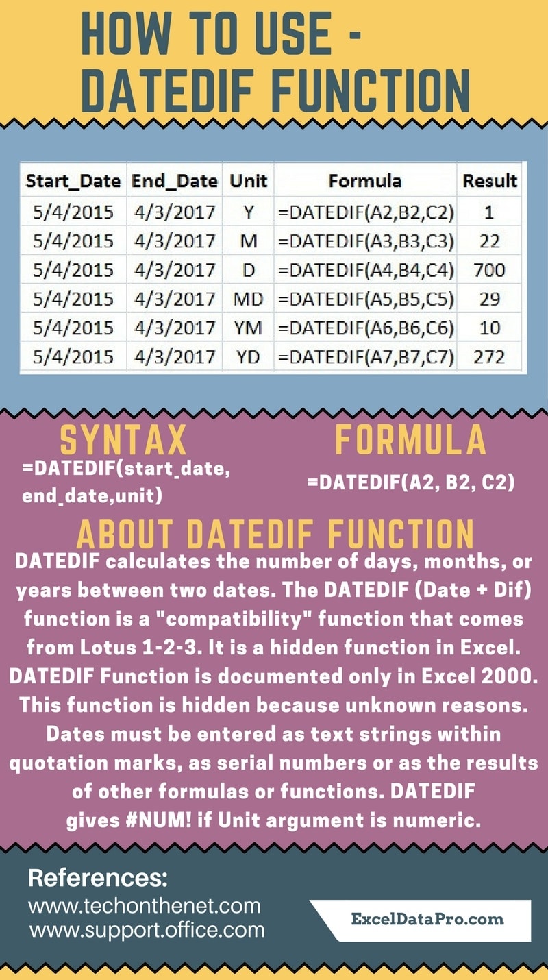
How To Use DATEDIF Function ExcelDataPro
Rumus DATEDIF yang pertama ini hanya akan menghitung selisih tahunnya saja, sisa bulan dan hari akan diabaikan. Hasil rumus DATEDIF dalam contoh yang pertama ini adalah 1 dan angka tersebut jika dihitung secara manual didapatkan dari : 2023 - 2022 = 1. Contoh yang kedua kita akan menghitung selisih tanggal dengan rumus DATEDIF dan satuan yang.
:max_bytes(150000):strip_icc()/FunctionExample-5bec4b96c9e77c0051918661.jpg)
Count Days, Months, Years With DATEDIF Function in Excel
Menghitung jumlah hari, bulan, atau tahun di antara dua tanggal. Peringatan: Excel menyediakan fungsi DATEDIF untuk mendukung buku kerja yang lebih lama dari Lotus 1-2-3. Fungsi DATEDIF mungkin menghitung hasil yang tidak benar di bawah skenario tertentu. Silakan lihat bagian masalah umum di artikel ini untuk detail selengkapnya.
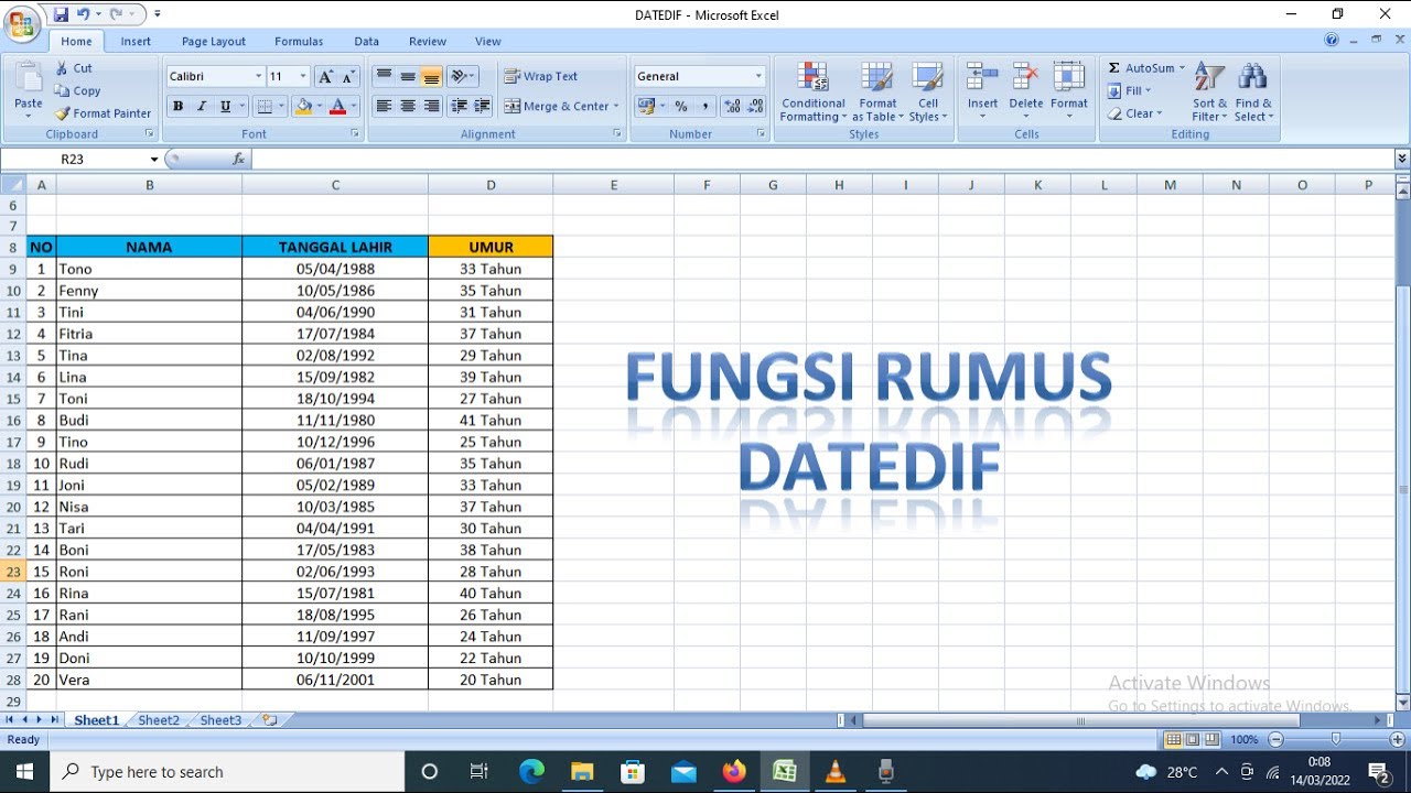
Rumus Datedif Excel, Cara Menghitung Umur/Usia di Microsoft Excel tutorialexcel belajarexcel
In the above example, Excel DATEDIF function returns the total number of days completed between 01 January 1990 and the current date (which is 14 March 2016 in this example). It returns 9569, which is the total number of days between the two dates. If you want to get the number of days between the two dates while excluding the ones from the.

Rumus Excel DATEDIF dan EDATE untuk menghitung selisih hari YouTube
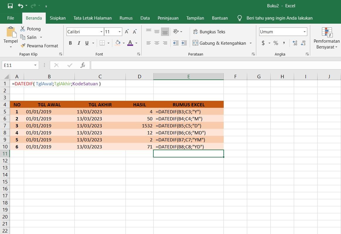
Pada rumus DATEDIF juga memiliki kode satuan dan ini merupakan sebuah Argumen yang berfungsi untuk mendapatkan informasi selisih tanggal di excel. Baca juga: Penggunaan Rumus IF di Excel. Argumen kode satuan tersebut seperti "Y", "M", "D", "MD", "YM", "YD". Pada Argumen Y untuk menghasilkan jumlah total tahun antara.

Rumus Cara Menghitung Umur Menggunakan Microsoft Excel Lengkap Dengan Tahun Bulan dan Hari
Gunakan fungsi DATEDIF ketika Anda ingin menghitung selisih antara dua tanggal. Pertama, masukkan tanggal mulai dalam sel, dan tanggal selesai di sel lain. Kemudian, ketikkan rumus seperti salah satu berikut ini. Peringatan: Jika Start_date lebih besar daripada End_date, hasilnya akan berupa #NUM!.

Rumus DATEDIF Excel (Cara & Contoh Fungsi DATEDIF di Excel)
Hallo teman-teman pada tutorial kali ini akan membahas tentang Belajar Rumus IF dan DATEDIF di Excel. Tutorial kali ini kita belajar penggunaan logika IF dan.

CARA PENGGUNAAN RUMUS FUNGSI TEXT & DATEDIF (Untuk Menghitung Usia) DI EXCEL Belajar Excel
To find out how many weeks there are between two dates, you can use the DATEDIF function with "D" unit to return the difference in days, and then divide the result by 7. To get the number of full weeks between the dates, wrap your DATEDIF formula in the ROUNDDOWN function, which always rounds the number towards zero:

Cara Menghitung Umur dengan Excel dari Tanggal Lahir Mengunakan rumus Datedif dan Year. YouTube
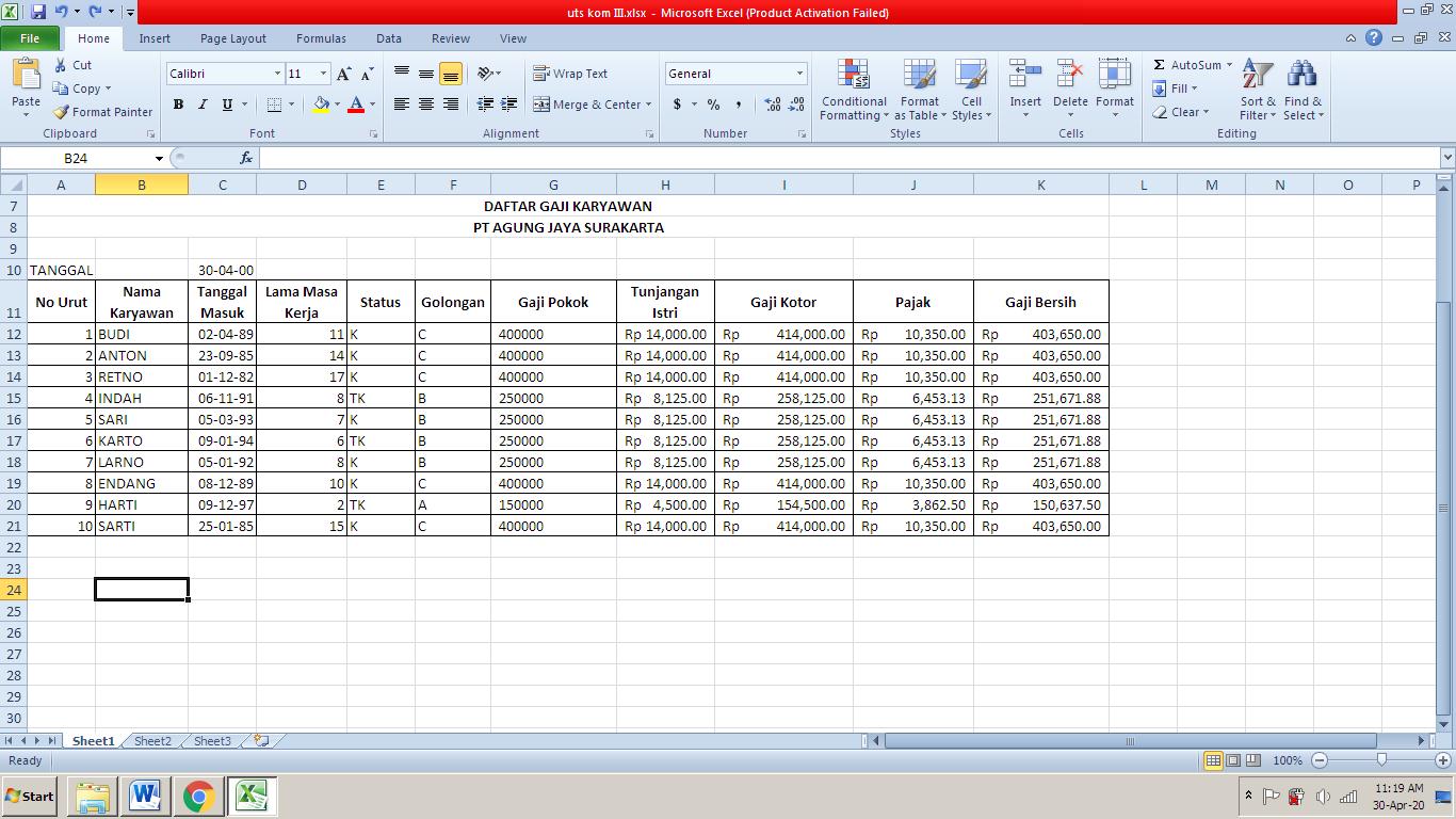
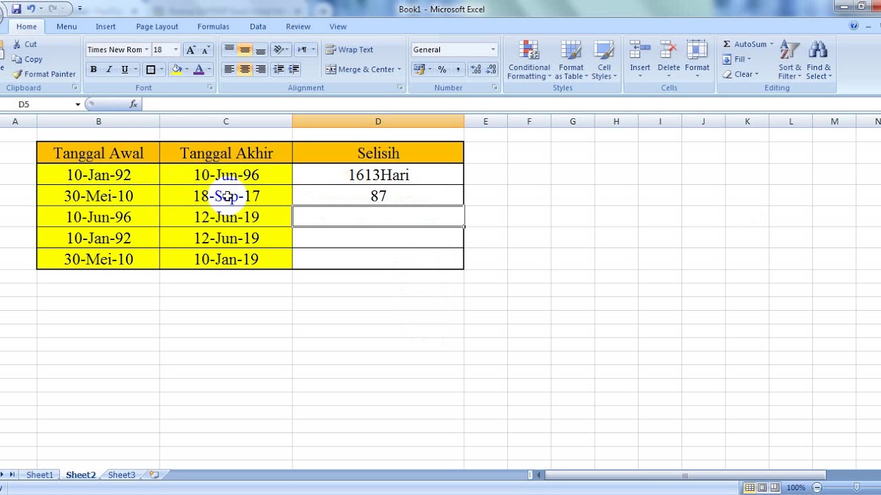
Formula DATEDIF digunakan untuk menghitung selisih hari, bulan, atau tahun dari dua tanggal yang diberikan. Untuk kebutuhan kerja, biasanya formula ini digunakan untuk menghitung umur atau masa kerja karyawan.. Dengan cara ketikkan rumus berikut. Karena ingin menghitung jumlah total hari maka kode satuan yang digunakan adalah "D". Dari.
CARA MENGGUNAKAN RUMUS DATEDIF DI EXCEL
DATEDIF is a versatile function that can be used in financial analysis, project planning, age calculation, and other scenarios that need to calculate time intervals in days, months, or years. The status of DATEDIF in Excel is somewhat mysterious. DATEDIF (Date + Dif) is a "compatibility" function that comes from Lotus 1-2-3 way back in the 1990s.
Rumus Datedif Excel Cara Menggunakan Rumus Datedif Excel Fungsi Contoh Dan Langkah Penulisan
Example 3. To count the number of whole months between dates, DATEDIF function with "M" unit can be used. The formula =DATEDIF (start_date, end_date, "m") compares the dates in A2 (start date) and B2 (end date) and returns the difference in months: Suppose we are given the following dates: The formula used is: The solution we get is:

Cara Menghitung Selisih Tanggal di Excel Kelas Excel Fungsi DATEDIF YouTube
Important note: the DATEDIF function returns the number of complete days, months or years. This may give unexpected results when the day/month number of the second date is lower than the day/month number of the first date. See the example below. The difference is 6 years. Almost 7 years! Use the following formula to return 7 years.
Hitung Masa Kerja di Excel Menggunakan Rumus Datedif YouTube
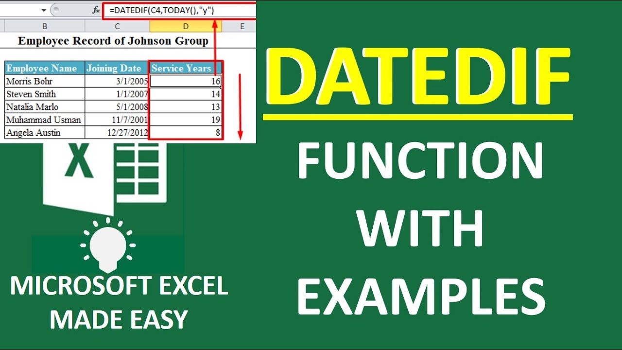
DATEDIF is a built-in Excel function that calculates the difference between two dates in various units, such as days, months, and years. (Source: Excel Easy) The syntax for the DATEDIF formula is "DATEDIF (start_date, end_date, unit)". (Source: Microsoft Excel) The "unit" argument can be "d" for days, "m" for months, or "y.
Rumus DATEDIF Excel Untuk Menghitung Selisih Tanggal YouTube
Fungsi DATEDIF, Rumus Excel untuk Menghitung Umur Rumus Excel [.] com - Untuk menghitung umur atau usia bisa menggunakan rumus excel DATEDIF. Fungsi DATEDIF digunakan untuk menghitung perbedaan/selisih antara dua tanggal dalam bentuk unit waktu tertentu. Fungsi ini tersedia pada aplikasi Microsoft Excel sejak versi 5/95 tetapi pada versi 2000 ke atas fungsi ini tidak di dokumentasikan dalam.
[EASY!] Excel DATEDIF Function With Examples How to Use The DATEDIF Function YouTube
Rumus DATEDIF di atas menghasilkan 1 karena sudah melewati satu tahun dari 1 November 2023 ke 28 Februari 2025, tapi tidak cukup panjang untuk dua tahun. Ingat. DATEDIF membulatkan hasil ke bawah, yaitu ke tahun penuh terdekat. Gambar 02. Menghitung selisih tahun di Excel menggunakan DATEDIF.

Cara Menghitung Durasi Waktu di Excel dengan Rumus Datedif YouTube
Add the TODAY function as the second parameter. DATEDIF in Google Sheets: Formula & Examples - Add TODAY Function. 3. Add "YM" as the third parameter, close the parenthesis, and press 'Enter'. DATEDIF in Google Sheets: Formula & Examples - Add "YM" Unit. 4. As you can see, the result is 11 months.

Rumus DATEDIF Excel Untuk Menghitung Selisih Tanggal YouTube
I am calculating Years of Service: =DATEDIF(C2,F2,"Y") but it is coming back with #NUM. I have both dates formatted with the 4 digit year (02/14/1972) in C2 and F2, which picks up today's date (both formatted the same). I also tried switching the formatting in the formula cell but nothing works.