
Cara Menggunakan Excel Conditional Formatting Tutorial Microsoft Excel YouTube
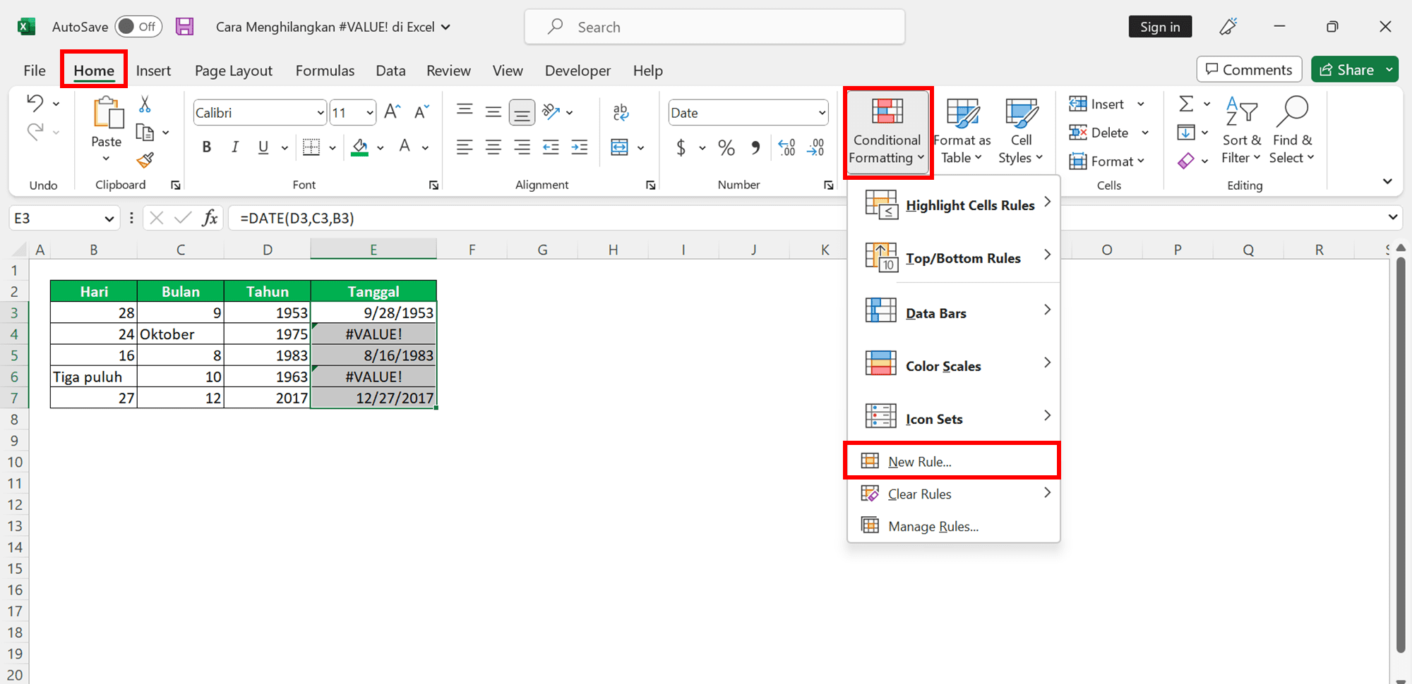
Step 1 Click on the "Conditional Formatting" button in the "Styles" group. Choose "New Rule" from the dropdown menu. Click new rule. Step 2 : In the "New Formatting Rule" dialog box, select "Use a formula to determine which cells to format." select Use a formula to determine which cells to format.

Cara Menghapus Format Warna Otomatis (Clear Conditional Formatting) Tutorial Singkat YouTube
Something as shown below: Here are the steps to create this Search and Highlight functionality: Select the dataset. Go to Home -> Conditional Formatting -> New Rule (Keyboard Shortcut - Alt + O + D). In the New Formatting Rule dialogue box, select the option 'Use a formula to determine which cells to format'.

Cara Menghapus Conditional Formatting Pada Excel YouTube
Ketika Anda menghapus format kondisional, Anda bisa memilih apakah menghapus format pada cell yang dipilih, keseluruhan sheet, PivotTable, atau tabel Excel. Cara menghapus format kondisional: Pilih cell yang memiliki format kondisional yang ingin Anda hapus. Klik tab Home. Pada grup Styles di Ribbon, klik Conditional Formatting. Arahkan ke.

Cara Menghilangkan Format Tabel Di Word IMAGESEE
Berikut beberapa panduan Conditional Formatting Excel Lainnya: Panduan Conditional Formatting Pada Microsoft Excel. Cara Memberi Warna Otomatis Sel yang Berisi Angka Tertentu. Cara Menandai Otomatis Sel yang Berisi Teks Tertentu. Cara Menemukan Data Ganda dan Data Unik Pada Excel. Cara Mewarnai Cell Dengan Rumus Excel.

How to Use Conditional Formatting in Microsoft Excel (2022)
adalah video yang menjelaskan tentang conditional formatting atau tutorial tentang bagaimana kita akan kupas tuntas conditional formatting di microsoft excel.
PART 2. CARA MENGHILANGKAN "N/A" DAN "VALUE" SERTA MENGGUNAKAN CONDITIONAL FORMATING DI MS
Namun, untuk menguasai cara menggunakan Conditional Formatting, Anda harus paham aturan penggunaannya terlebih dahulu. Untuk itu, Panduan ini Saya susun sebagai teknik dasar penggunaan Conditional Formatting. Jika Anda sudah paham teknik dasar ini, silahkan masuk ke SUB-BAB selanjutnya untuk memantapkan kemampuan Anda..
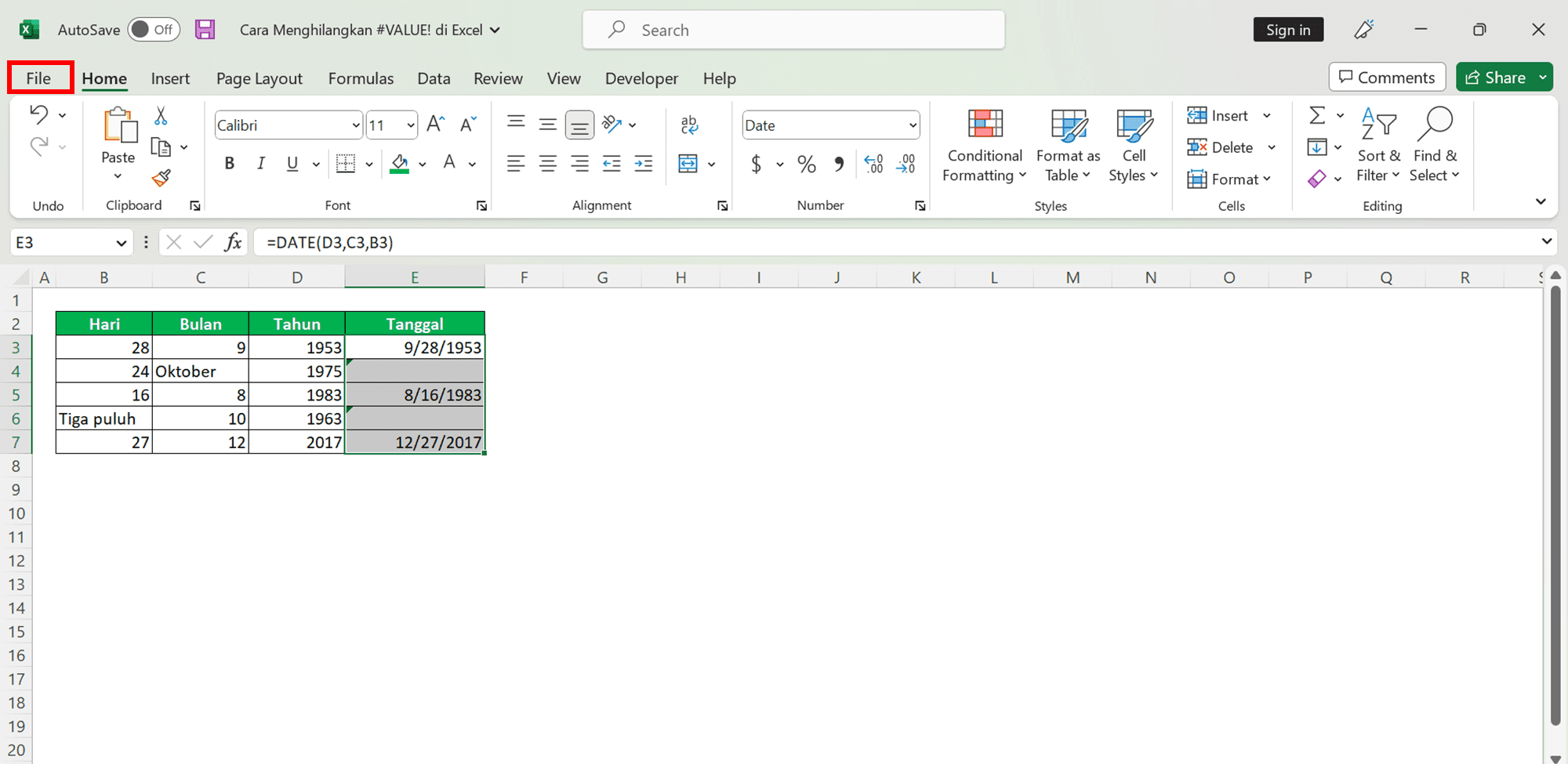
Cara Menghilangkan VALUE! di Excel Compute Expert
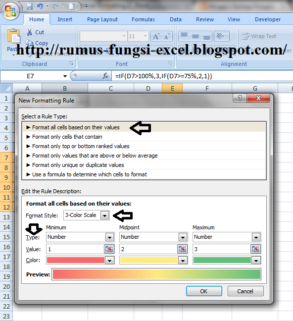
Pilih sel yang ingin diterapkan format kondisional. Klik perintah Conditional Formatting. Sebuah menu drop-down akan muncul. Arahkan mouse pada preset yang diinginkan, kemudian memilih gaya yang telah ditetapkan dari menu yang muncul. Format kondisional akan diterapkan pada sel yang dipilih.
Cara Membuat Rules Warna Excel Warga.Co.Id
Jika ingin menghapus dengan cara ini maka ikuti langkah - langkah dibawah ini : - Pilih/blok range yang akan dihapus. - Klik Home. - Klik Conditional Formatting. - Klik Clear Rules. Setelah klik Clear Rules ada 4 pilihan yang muncul yaitu : Clear rules from selected cells : Conditional Formatting yang dihapus hanya pada cell/range yang dipilih.

🔴TIPS EXCEL Cara Membuat CONDITIONAL FORMATTING, menggunakan rumus IF dan MATCH YouTube
Panel ini akan mengarahkan bagaimana menerapkan format bersyarat ke sel di Google Sheets. Hal yang perlu diperhatikan adalah setiap baris harus memiliki logika yang diperlukan untuk menentukan bagaimana memperlakukan sel berdasarkan isinya. 2. Cara Memformat Sel di Google Sheets Menggunakan Pemformatan Bersyarat.
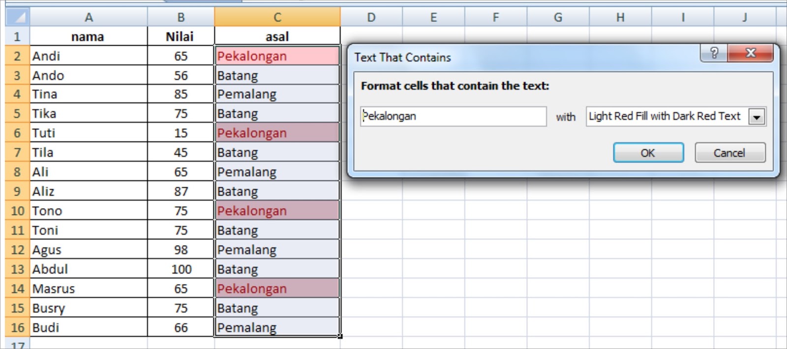
Conditional formatting text that contains Belajar Microsoft Office dan Bahasa Inggris
Untuk menghapus pemformatan bersyarat rentang yang dipilih, lakukan seperti ini: 1. Pilih rentang yang ingin Anda hapus pemformatan bersyarat. 2. Klik Beranda > Format Bersyarat > Aturan yang Jelas > Hapus Aturan dari Sel yang Dipilih. Lihat tangkapan layar: 3. Dan pemformatan bersyarat yang dipilih telah dihapus. Lihat tangkapan layar:

Beberapa jenis Conditional formatting pada ms.excel dan cara menghilangkannya / menghapusnya
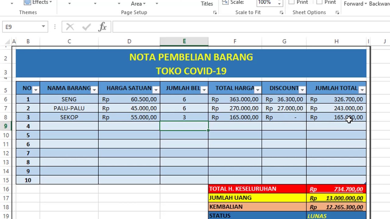
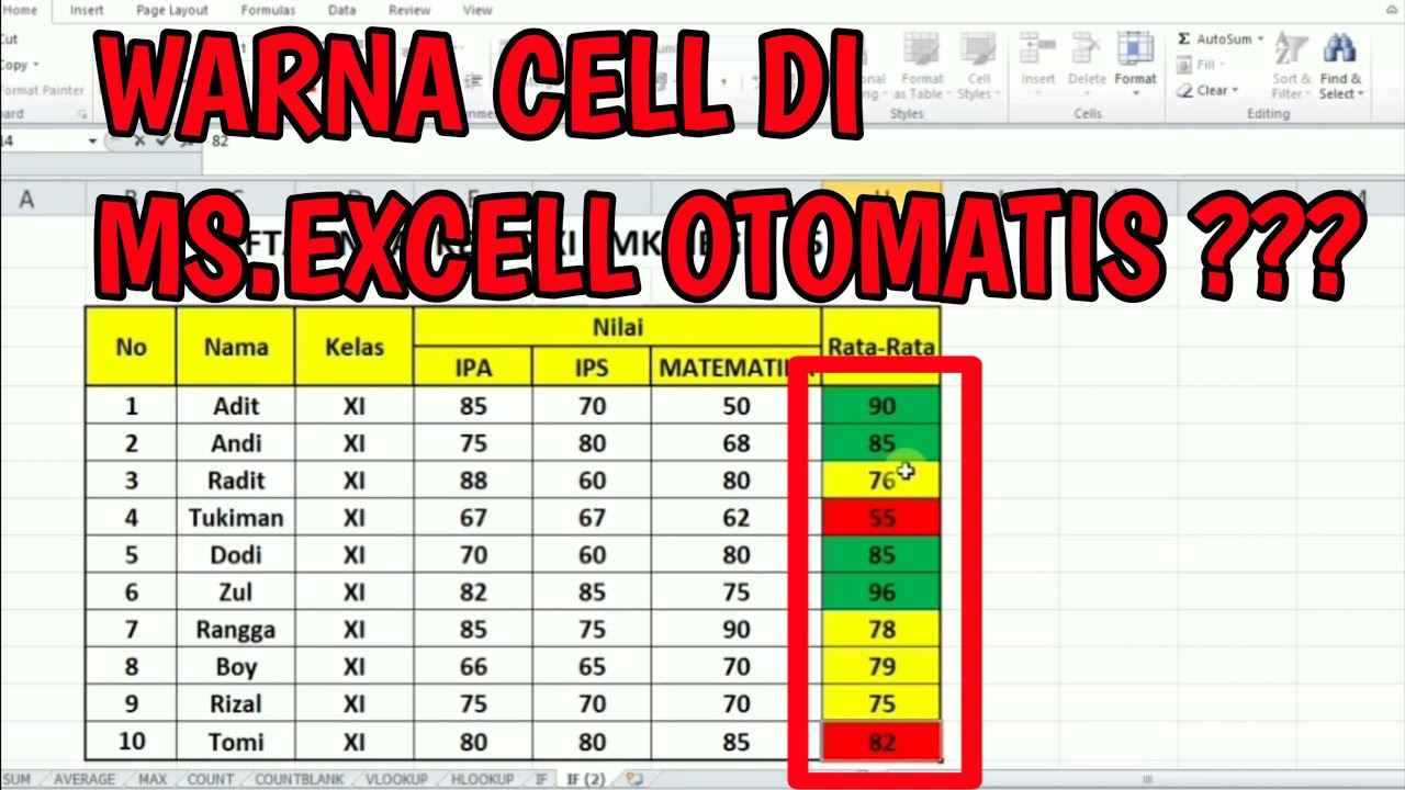
Klik Use a formula to determine which cells to format. Dalam kotak Format values where this formula is true masukan rumus : =IF (B4<=60;1;0) Klik tombol Format dan akan muncul kotak dialog Format Cells. Dalam kotak dialog Format Cells klik Tab Fill. Klik warna yang akan digunakan pada kelompok menu Background Color.
Cara Menggunakan Conditional Formatting Dengan Rumus If Perhitungan Soal
Hi, Please check whether the following solution is helpful: Step 1) Select the 1st date in the date column. Step 2) Select all the dates in the date column. Step 3) In Home tab >> click on Conditional Formatting drop-down >> click on New Rule >> for 1st Rule, type the formula as illustrated in the 1st screenshot. Step 4) Apply formatting. Step 5) Click on OK.-Repeat the Steps for all rules.

Cara Conditional Formating di Google Sheets (Memberi Warna Pada Huruf dan Angka Tertentu) YouTube
2. Create a conditional formatting rule, and select the Formula option. 3. Enter a formula that returns TRUE or FALSE. 4. Set formatting options and save the rule. The ISODD function only returns TRUE for odd numbers, triggering the rule: Video: How to apply conditional formatting with a formula.
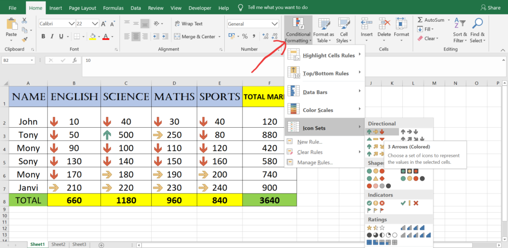
ICON SETS In Conditional Formatting ExcelHelp
Without conditional formatting: With conditional formatting: Removing Conditional Formatting. To remove conditional formatting from a single cell or range, follow these steps. Step 1. Select the cell or range you want to remove conditional formatting from. Step 2. Open the Format menu, then click on the Conditional Formatting option. Step 3

CARA MEMBUAT CONDITIONAL FORMATTING DI EXCEL Warga.Co.Id
Video ini berisi :3 Cara Panduan Menghapus Conditional Formatting pada Excelcara menghapus conditional formatting pada excel, cara menghilangkan conditional.
Cara Menghilangkan VALUE! di Excel Compute Expert
Clear Rules from This PivotTabel: Menghapus conditional formatting pada pivot tabel terpilih saja. Cara II: Menghilangkan Conditional Formatting Melalui Manage Rule. Pilih cell/range data, tabel atau PivotTable yang ingin dihapus condittional formatting-nya. Pilih Tab Home-Conditional Formatting-Manage Rules.